Neurochat API guide
In addition to the codes for verifying the place cell, head-directional cell and analyses of rhythmic units, it also shows examples of other useful methods that can be harnessed for creating simple and efficient analysis scripts and data management.
Please refer to the code-documentation for the description of each module, their classes and functions, and methods in each class.
In addition to the example units, this guide shows uses of NeuroChaT and its components in many different ways.
Step 1: Install NeuroChaT
[1]:
python -m pip install neurochat
Step 2: Import modules and classes
We are importing only NSpike and NSpatial for the moment. We will add and import NLfp data for analyses that require LFP signals. nc_plot is the module that provides with plotting functions
[2]:
from neurochat.nc_data import NData
from neurochat.nc_spike import NSpike
from neurochat.nc_spatial import NSpatial
import neurochat.nc_plot as nc_plot
Step 3: Instantiate objects
The names C0 and S0 for for the unit and the spatial data are arbitrary
[3]:
spike = NSpike(system='Axona')
spike.set_name('C0')

spat = NSpatial(system='Axona')
spat.set_name('S0')
Step 4: Add paths to the data files
[4]:
data_dir= 'C:\\Users\\Raju\\Google Drive\\Sample Data for NC\\Place Cell\\Place cell 6 tetrode 6 cluster 3\\'

spat.set_filename(data_dir + '040513_1_1.txt')
spike.set_filename(data_dir + '040513_1.6')
Step 4a: For HDF5 files
Path of the data should also be added following a ‘+’ sign. The system argument should be changed or could be set at NSpatial(system=Axona')
[ ]:
spat.set_system('NWB')
spike.set_system('NWB')

data_dir = 'C:\\Users\\Raju\\Google Drive\\Sample Data for NC\\Place Cell\\Place cell 6 tetrode 6 cluster 3\\'
spat.set_filename(data_dir + '040513_1.hdf5+/processing/Behavioural/Position')
spike.set_filename(data_dir + '040513_1.hdf5+/processing/Shank/6')
Step 5: Load spatial and spike data and set the unit number
[5]:
spat.load()
spike.load()

spike.set_unit_no(3)
Step 6: Instantiate NData object. Add individual data objects to NData object.
[6]:
ndata = NData()
ndata.spike = spike
ndata.spatial = spat
The data format, filenames for individual datasets can be set using ndata
[ ]:
ndata.set_data_format(data_format='NWB')

ndata.set_spatial_file(data_dir + '040513_1.hdf5+/processing/Behavioural/Position')
ndata.set_spike_file(data_dir + '040513_1.hdf5+/processing/Shank/6')
They can be loaded using ndata
[ ]:
ndata.load()
Or, individually
[ ]:
ndata.load_spatial()
ndata.load_spike()
And the unit number can be set as well
[ ]:
ndata.set_unit_no(3)
Step 8: Perform analysis of interest
Step 8a: Analysis of a place cell
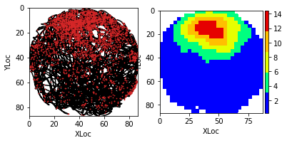
Place cell firing map by using ndata: Pixel size is set 3cm. A 5x5 box filter is used for smoothing the firing map
[7]:
placeData = ndata.place(pixel=3, filter=['b', 5])
Alternative place cell call
Similar results can be obtained by passing timestamps of the spiking unit to the spat.place() method NData object performs the job of connecting these two objects and simplifies the analysis
[ ]:
placeData = spat.place(spike.get_unit_stamp(), pixel=3, filter=['b', 5])
Plotting relevant data
Refer to nc_plot.py module for more plotting functions.
Following command is used for inline display of graphics in Notebook
[8]:
%matplotlib inline
[9]:
fig = nc_plot.loc_firing(placeData)
Locational shuffling analysis
By default, the spike timestamps are shuffled for 500 times. Pixel size is 3 cm. limit=0 implies that the spikes timestamps are randomly shuffled in (-duration, +duration) range
[10]:
pshuffleData = ndata.loc_shuffle(nshuff=500, limit=0, pixel=3)
fig = nc_plot.loc_shuffle(pshuffleData)
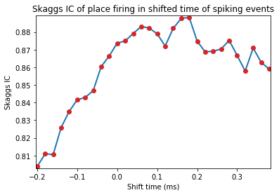
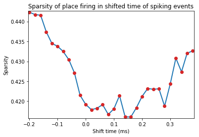
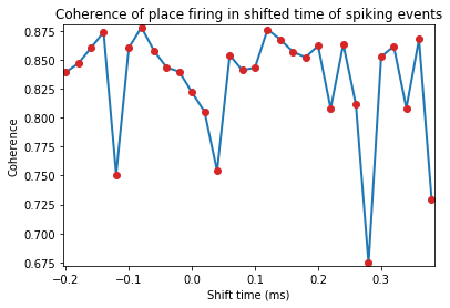
Locational shifting analysis
Spike timestamps are gradually shifted from -10 to +20 units of spatial time-resolution. If the video for tracking animal behviour is sampled at 50Hz, this means the spike-train is shifted from -200ms to +400ms
[11]:
import numpy as np # numpy imported for the use of np.range
pshiftData = ndata.loc_shift(shift_ind=np.arange(-10, 20))
fig = nc_plot.loc_time_shift(pshiftData)
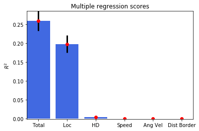
Multiple regression analysis
[13]:
regressData = ndata.multiple_regression()
fig = nc_plot.multiple_regression(regressData)
Exporting data to NWB format
If the data files are in Axona or Neuralynx format, they can be exported to HDF5 file
[ ]:
ndata.save_to_hdf5()
Datasets can be saved individually as well
[14]:
spike.save_to_hdf5()
spat.save_to_hdf5()
Print parametric results of all analyses performed
[15]:
results = ndata.get_results() # Returns the results in OrderedDict
print(results)
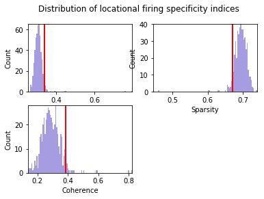
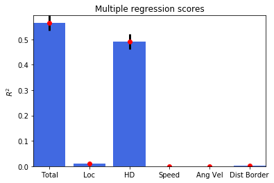
OrderedDict([('Spatial Skaggs', 0.87363237668517801), ('Spatial Sparsity', 0.41920352222017176), ('Spatial Coherence', 0.82191292689890405), ('Loc Skaggs 95', 0.33743438803043752), ('Loc Sparsity 05', 0.71946056545786297), ('Loc Coherence 95', 0.38296777900374684), ('Loc Opt Shift Skaggs', array([ 0.18])), ('Loc Opt Shift Sparsity', array([ 0.16])), ('Loc Opt Shift Coherence', array([-0.08])), ('HD Skaggs', 0.17060729747597284), ('HD Rayl Z', 24.493680532080919), ('HD Rayl P', 1.2819522146275648e-11), ('HD von Mises K', 0.6639255940574873), ('HD Mean', 137.54600963832547), ('HD Mean Rate', 77.748719154002572), ('HD Res Vect', 0.31503645074286685), ('HD Peak Rate', 7.5858250276854937), ('HD Peak', 115), ('HD Half Width', 176), ('Mult Rsq', 0.2587727606182223), ('Semi Rsq Loc', 0.19786047209173907), ('Semi Rsq HD', 0.0049837182830173334), ('Semi Rsq Speed', 0.00078688801150850391), ('Semi Rsq Ang Vel', 0.0005234149863417505), ('Semi Rsq Dist Border', 0.00048427333149445273)])
Results from individual data objects can be retrieved similarly
[ ]:
spike_results = spike.get_results()
spat_results = spat.get_results()
## Step8b: Analysis of a head-directional cell Change data filename/paths for the new unit similar to what was done for the place cell information Load new data and set the unit number. No need to reassign to ndata, as Python assignments are by reference, not by value.
[16]:
ndata.set_data_format('NWB')
data_dir = 'C:\\Users\\Raju\\Google Drive\\Sample Data for NC\HD Cell\\HD cell tetrode 3 Cluster 1\\'
spat.set_filename(data_dir + '120412_1.hdf5+/processing/Behavioural/Position')
spike.set_filename(data_dir + '120412_1.hdf5+/processing/Shank/3')
spat.load()
spike.load()
spike.set_unit_no(1)
Reset results to omit parametric output of previously analysed unit. This can be done before loading the new datasets or at any stage of the analysis.
[17]:
ndata.reset_results()
Or, results can be reset using individual data objects
[ ]:
spat.reset_results()
spike.reset_results()
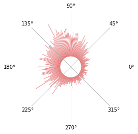
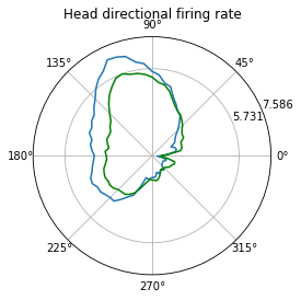
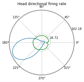
Head-directional firing rate analysis
[18]:
hdData = ndata.hd_rate()
fig = nc_plot.hd_firing(hdData)
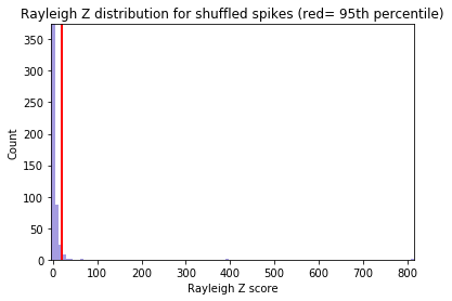
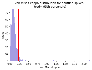
Head directional shuffling analysis
The number of bins for the histogram of the shuffled data is set to 100
[19]:
hshuffleData = ndata.hd_shuffle(nshuff=500, limit=0, bins=100)
fig = nc_plot.hd_shuffle(hshuffleData)
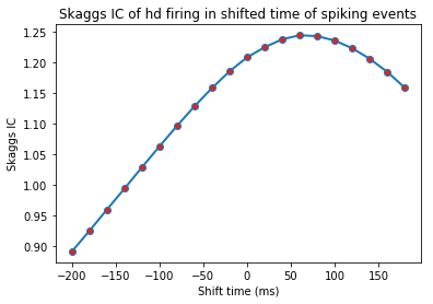
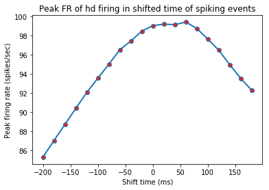
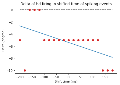
Head directional time-shift analysis
[20]:
hshiftData = ndata.hd_shift(shift_ind=np.arange(-10, 10))
fig = nc_plot.hd_time_shift(hshiftData)
Head directional multiple regression
[21]:
regressData = ndata.multiple_regression()
fig = nc_plot.multiple_regression(regressData)
Step 8c: Analysis of spike-train dynamics
Changing the data filename/paths for the new unit
[22]:
data_dir= 'C:\\Users\\Raju\\Google Drive\\Sample Data for NC\\Theta cell tetrode 5 Cluster 1\\'
spat.set_filename(data_dir + '112512_1.hdf5+/processing/Behavioural/Position')
spike.set_filename(data_dir + '112512_1.hdf5+/processing/Shank/5')

spat.load()
spike.load()

spike.set_unit_no(1)
Reset results to omit parametric output of previously analysed unit
[23]:
ndata.reset_results()
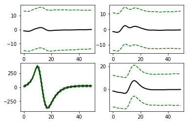
Waveform properties of the unit
[24]:
graphData = ndata.wave_property()
fig = nc_plot.wave_property(graphData, [int (spike.get_total_channels()/2), 2])
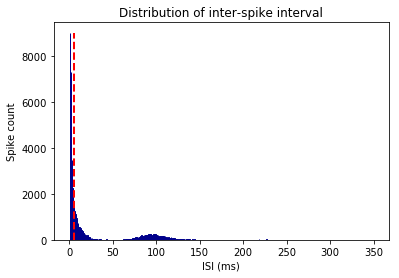
Inter-spike interval (ISI) histogram.
The number of bins for histogram is 350, and the maximum ISI to bin for is 350ms. This implies each bin represents 1msec interval. ‘graphData’ term will be used repetedly from now on for reusing the memory
[25]:
graphData = ndata.isi(bins=350, bound=[0, 350])
fig = nc_plot.isi(graphData)
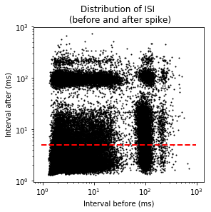
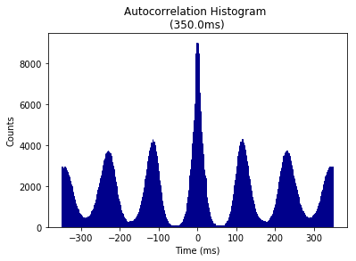
ISI autocorrelation histogram for longer length
Binsize is 1msec, and autocrrelation is performed from -350ms to +350ms
[26]:
graphData = ndata.isi_corr(bins=1, bound=[-350, 350])
fig = nc_plot.isi_corr(graphData)
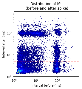
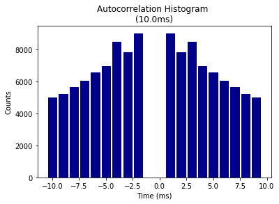
ISI autocorrelation histogram for shorter length
Binsize is 1msec, and autocrrelation is performed from -10ms to +10ms
[27]:
graphData = ndata.isi_corr(bins=1, bound=[-10, 10])
fig = nc_plot.isi_corr(graphData)
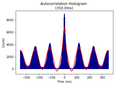
Theta modulation Index analysis
Input parameters are for [Frequency, tau1, tau2] and provides the starting value, lower, and upper bound for the fitted sinusoidal equation. Binsize and remporal bound are that of ISI autocorrelation histogram
[28]:
graphData = ndata.theta_index(
    start = [6, 0.1, 0.05],
    lower = [4, 0, 0],
    upper = [14, 5, 0.1],
    bins = 1, bound = [-350, 350])
fig = nc_plot.theta_cell(graphData)
Above analyses can also be done using the spike data itself as it does not require information from other data object. For example,
[ ]:
graphData = spike.isi(bins=350, bound=[0, 350])
fig = nc_plot.isi(graphData)
Step 8d: Analysis of rhythmicity of LFP and spike-to-LFP phase relationships
Import NLfp class
[30]:
from neurochat.nc_lfp import NLfp
Instatiate LFP data object, set the filename, load data, and add to ndata
[31]:
lfp = NLfp(system='NWB')

lfp.set_filename(data_dir+ '\\112512_1.hdf5+/processing/Neural Continuous/LFP/eeg')

lfp.load()

ndata.lfp = lfp
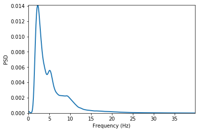
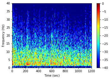
LFP frequency spectrum analysis
Hanning window of 2sec with 1sec overlap and number of FFT components = 2048. ptype is ‘psd’ which means power-spectral density. Other option can be ‘power’. prefilt set ‘True’ for pre-filtering the LFP signal with a bandpass filter as set by filtset.
filtset = [
    filter order, lower cutoff frequency,
    higher cutoff frequency, type of filtering]
fmax defines the maximum frequency to analyse. db set to ‘True’ will convert the spectogram in decibel unit. tr set to ‘True’ creates a time-resolved spectogram with ‘window’-resolution and ‘overlap’ amount of signal overlap. tr set to ‘False’ calculates the spectogram using Welch’s method. This function can also be similarly called as ndata.spectrum()
[32]:
graphData = lfp.spectrum(
    window=2, noverlap=1, nfft=2048, ptype='psd',
    prefilt=True, filtset=[10, 1.5, 40, 'bandpass'],
    fmax=40, db=False, tr=False)
fig = nc_plot.lfp_spectrum(graphData)
After setting tr as True and db = True
[33]:
graphData= lfp.spectrum(
    window=2, noverlap=1, nfft=2048, ptype='psd',
    prefilt=True, filtset=[10, 1.5, 40, 'bandpass'],
    fmax=40, db=True, tr=True)
fig = nc_plot.lfp_spectrum_tr(graphData)
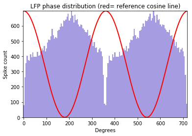
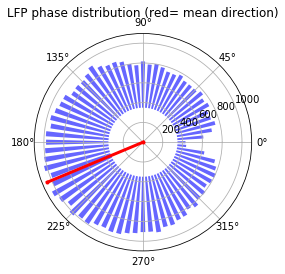
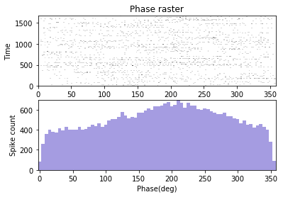
Spike-LFP phase distribution
fwin = [6,12] means that the phase of the spike are sought in the LFP band of 6Hz to 12 Hz. The minimum power of this band to be accepted to carry significant theta is 0.2 times the total LFP power, and that of the amplitude of the band signal is 0.15 times the amplitude of the LFP signal. The LFP signal is prefiltered using the filtset parameters.
[34]:
graphData = ndata.phase_dist(
    binsize=5, rbinsize=2, fwin=[6, 12],
    pratio=0.1, aratio=0.15, filtset=[10, 1.5, 40, 'bandpass'])
fig = nc_plot.spike_phase(graphData)
The analysis can be performed from both the NLfp() and NSpike() objects
Using the lfp object:
[ ]:
graphData = lfp.phase_dist(
    spike.get_unit_stamp(), binsize=5, rbinsize=2, fwin=[6, 12],
    pratio=0.1, aratio=0.15, filtset=[10, 1.5, 40, 'bandpass'])
fig= nc_plot.spike_phase(graphData)
Using the spike object:
[ ]:
graphData = spike.phase_dist(
    lfp=lfp , binsize=5, rbinsize=2, fwin=[6, 12],
    pratio=0.1, aratio=0.15, filtset=[10, 1.5, 40, 'bandpass'])
fig= nc_plot.spike_phase(graphData)
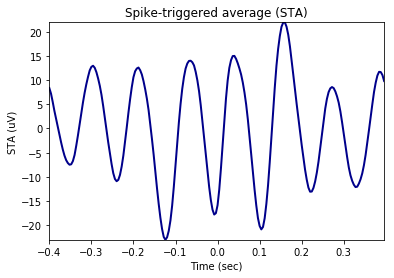
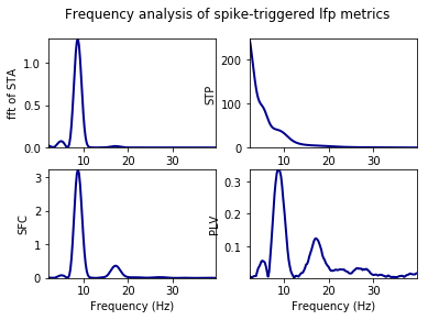
Analysis of phase-locking value (PLV), spike-field coherence (SFC), and spike-triggerd average (STA)
Window of the LFP chunks in reference to the spike timestamps is set to -400ms to +400ms Frequency of interest for the analysis is set as 2Hz to 30Hz
[35]:
graphData = ndata.plv(window=[-0.4, 0.4], fwin=[2, 40])
fig = nc_plot.plv(graphData)
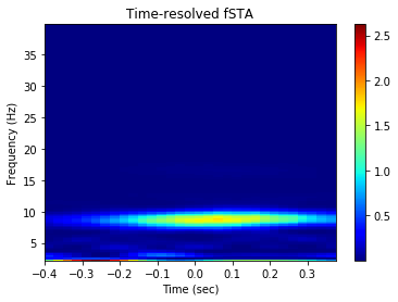
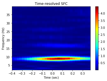
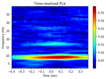
Time-resolved as set by mode= ‘tr’. nsample implies number of randomly selected spikes around which the LFP signals are cut for phase-locking analysis slide gives the time in ms by which the window is shifted from left to right to obtain the time-resolved phase-locking analysis
[36]:
graphData = ndata.plv(
    window=[-0.4, 0.4], nfft=1024, mode='tr',
    nsample=2000, slide=25,fwin=[2, 40])
fig = nc_plot.plv_tr(graphData)
In most of the cases where composite information are required and ndata is not used, the spike timestamp is provided as the first argument to the methods followed by other information. Because, in such cases only information required by the analysis from the spike object is the timestamps of individual spikes in the train. For example,
[ ]:
graphData = ndata.plv(window=[-0.4, 0.4], fwin=[2, 40])
fig = nc_plot.plv(graphData)
gives the same result as the codes given below:
[ ]:
graphData = lfp.plv(
    spike.get_unit_stamp(), window=[-0.4, 0.4], fwin=[2, 30])
fig = nc_plot.plv(graphData)
Step 9: Using the Nhdf class
Import and instantiate Nhdf class
[37]:
from neurochat.nc_hdf import Nhdf
hdf = Nhdf()
Store data using Nhdf object
Nhdf() resolves the filename and the path for storage of the data using Nhdf().resolve_pathname(data=data_obj) where data_obj can be a NSpatial(), NSpike() of NLfp() object
[38]:
hdf.save_spatial(spat)
hdf.save_spike(spike)
hdf.save_lfp(lfp)
This can also be done using
[ ]:
hdf.save_object(obj=spat)
hdf.save_object(obj=spike)
hdf.save_object(obj=lfp)
Graphical data from indiviudal analysis can be stored using the following codes.
path is the path inside HDF5 file. Analysis data are always recommended to store in the /analysis/ path. But analysis for each unit+lfp pair is stored in one path under which graphical data from individual analyses are store. The unique unit ID is established using the name resolving method Nhdf().resolve_analysis_path() which utilizes the filename of the recorded data, electrode/tetrode number, eeg channel ID and the unit number. name is the name of the analysis following the unit ID, i.e. ‘plv’ etc. graph_data are the dictionary data that are plotted using the functions iin nc_plot
[39]:
unit_id = hdf.resolve_analysis_path(spike=spike, lfp=lfp)

hdf_name = hdf.resolve_hdfname(data=spike) # Resolve HDF5 filename
hdf.set_filename(hdf_name) # NeuoChaT opens the file as file-object as soon as new filename is set.

print(unit_id)

hdf.save_dict_recursive(
    path ='/analysis/' + unit_id+ '/' ,
    name = 'plv', data = graphData)
TT5_SS_1_eeg
Analysis results can be stored by
[40]:
results = ndata.get_results()
hdf.save_dict_recursive(
    path='/analysis/' + unit_id+ '/' ,
    name='results', data=results)
Apart from that data and attributes to any group or dataset can be added using
Set create_group to ‘True’ it will create the path if does not already exist
[ ]:
hdf.save_dataset(
    path='/path/to/group/', name='name_of_dataset',
    data=date_to_store, create_group=True)
hdf.save_attributes(
    path='/path/to/group/or/dataset/',
    attr=dict_of_attributes)
Step 10: Use of NeuroChaT class
Import NeuroChaT class and instantiate
[41]:
from neurochat.nc_control import NeuroChaT
nc= NeuroChaT()
Convert files in Axona format to NWB files specified in an Excel list
[44]:
excel_file = 'C:\\Users\\Raju\\Google Drive\\Sample Data for NC\\Conversion list in this folder_labpc.xlsx'
nc.convert_to_nwb(excel_file)
:02:18:25 (nc_control.py)  --  Converting file groups: 1
:02:18:37 (nc_control.py)  --  Converting file groups: 2
:02:18:44 (nc_control.py)  --  Converting file groups: 3
:02:18:47 (nc_control.py)  --  Converting file groups: 4
:02:18:57 (nc_control.py)  --  Converting file groups: 5
:02:19:05 (nc_control.py)  --  Conversion process completed!
Verify units provided in an Excel list before batch-mode analysis
[46]:
excel_file = 'C:\\Users\\Raju\\Google Drive\\Sample Data for NC\\Verify unit list in this folder_labpc.xlsx'
nc.verify_units(excel_file)
:02:20:07 (nc_control.py)  --  Verifying unit: 1
:02:20:07 (nc_control.py)  --  Verifying unit: 2
:02:20:08 (nc_control.py)  --  Verifying unit: 3
:02:20:08 (nc_control.py)  --  Verifying unit: 4
:02:20:10 (nc_control.py)  --  Verifying unit: 5
:02:20:11 (nc_control.py)  --  Verification process completed!
Evaluate the quality of clustering from a list provided in an Excel file
[48]:
excel_file = 'C:\\Users\\Raju\\Google Drive\\Sample Data for NC\\Cluster quality evaluation unit list in this folder_labpc.xlsx'
nc.cluster_evaluate(excel_file)
:02:21:35 (nc_control.py)  --  Evaluating unit: 1
:02:21:38 (nc_control.py)  --  Evaluating unit: 2
:02:21:39 (nc_control.py)  --  Evaluating unit: 3
:02:21:51 (nc_control.py)  --  Cluster evaluation completed!
Evaluate similarity of clusters
The excel list contains paired list of units to be compared for similarity
[49]:
excel_file = 'C:\\Users\\Raju\\Google Drive\\Sample Data for NC\\Comparison results_from NeuroChaT_pawels_data.xlsx'
nc.cluster_evaluate(excel_file)
:02:22:47 (nc_control.py)  --  Evaluating unit: 1
:02:22:47 (nc_control.py)  --  Evaluating unit: 2
:02:22:47 (nc_control.py)  --  Evaluating unit: 3
:02:22:48 (nc_control.py)  --  Evaluating unit: 4
:02:22:48 (nc_control.py)  --  Evaluating unit: 5
:02:22:48 (nc_control.py)  --  Cluster evaluation completed!
Analysis using NeuroChaT
Analysis using NeuroChaT class is always done with the help of Configuration class where the user specifies all the data, intended analyses, input parameters etc.
Configuration class
Import, instantiate, set the filename and load configuration from the file. This class uses nc_defaults.py module for importing deafult analyses and parameters.
[54]:
from neurochat.nc_config import Configuration

config = Configuration()

config.set_config_file('C:\\Users\\Raju\\Google Drive\\Sample Data for NC\\grid_config.ncfg')

config.load_config()
Set configuration to NeuroChaT object
[55]:
nc.set_configuration(config)
Start analysis. This will ‘read’ the instructions from the config object and execute accordingly
[56]:
nc.start()
:02:24:45 (nc_control.py)  --  Starting a new unit...
:02:24:49 (nc_control.py)  --  Calculating environmental border...
:02:24:49 (nc_control.py)  --  Assessing waveform properties...
:02:24:52 (nc_control.py)  --  Calculating inter-spike interval distribution...
:02:24:55 (nc_control.py)  --  Calculating inter-spike interval autocorrelation histogram...
:02:25:03 (nc_control.py)  --  Estimating theta-modulation index...
:02:25:26 (nc_control.py)  --  Estimating theta-skipping index...
:02:25:32 (nc_control.py)  --  Analyzing bursting property...
:02:25:32 (nc_control.py)  --  Calculating spike-rate vs running speed...
:02:25:33 (nc_control.py)  --  Calculating spike-rate vs angular head velocity...
:02:25:33 (nc_control.py)  --  Assessing head-directional tuning...
:02:25:34 (nc_control.py)  --  Shuffling analysis of head-directional tuning...
:02:25:50 (nc_control.py)  --  Time-lapsed head-directional tuning...
:02:25:52 (nc_control.py)  --  Time-shift analysis of head-directional tuning...
:02:25:54 (nc_control.py)  --  Assessing of locational tuning...
:02:25:55 (nc_control.py)  --  Shuffling analysis of locational tuning...
:02:26:02 (nc_control.py)  --  Time-lapse analysis of locational tuning...
:02:26:07 (nc_control.py)  --  Time-shift analysis of locational tuning...
:02:26:08 (nc_control.py)  --  Spatial and rotational correlation of locational tuning...
C:\Users\Raju\Google Drive\NeuroChaT Py\neurochat\neurochat\nc_utils.py:289: RuntimeWarning: invalid value encountered in double_scalars
  np.sqrt(np.sum((x1- x1.mean())**2)*np.sum((x2- x2.mean())**2))
:02:26:09 (nc_control.py)  --  Assessing gridness...
:02:26:10 (nc_control.py)  --  Multiple-regression analysis...
:02:26:24 (nc_control.py)  --  Assessing dependence of variables to...
:02:26:26 (nc_control.py)  --  Output graphics saved to C:\Users\Raju\Google Drive\Sample Data for NC\Grid Cell\Grid cell tetrode 6 cluster 4\120213_26_TT6_SS_4_eeg.pdf
ERROR:02:26:26 (nc_hdf.py)  ERROR--  Error in creating HD ATI dataset to hdf5 file
:02:26:28 (nc_control.py)  --  Units already analyzed = 1
:02:26:28 (nc_control.py)  --  Total cell analyzed: 1
Use get_ and set_ functions also known as getters and setters for accessing and setting values of interest. For example,
### Getting and setting parameters:
[58]:
param_list = config.get_param_list() # List of all parameters as dictionary keys

params_by_analysis = config.get_params_by_analysis(analysis='isi')
print(params_by_analysis)

param_val = config.get_params(name='isi_length') # name is the list of parameters or the name of a single parameter'
print(param_val)

config.set_param(name='isi_bin', value=2)
{'isi_bin': 2, 'isi_length': 200}
200
Getting and setting analyses:
[61]:
list_of_analyses = config.get_analysis_list() # List of all analysis
print(list_of_analyses)

analysis_checked = config.get_analysis(name='isi') # If 'True', analysis is set to be done
print(analysis_checked)

config.set_analysis(name='theta_skip_cell', value=False) # Analysis of theta skipping cell turned off
['wave_property', 'isi', 'isi_corr', 'theta_cell', 'theta_skip_cell', 'burst', 'speed', 'ang_vel', 'hd_rate', 'hd_shuffle', 'hd_time_lapse', 'hd_time_shift', 'loc_rate', 'loc_shuffle', 'loc_time_lapse', 'loc_time_shift', 'spatial_corr', 'grid', 'border', 'gradient', 'multiple_regression', 'inter_depend', 'lfp_spectrum', 'spike_phase', 'phase_lock', 'lfp_spike_causality']
True
Analyses can be performed in different modes, namely: 1. ‘Single Unit’- one cell at time, value ‘0’ 2. ‘Single Session’- all the cells in one recording at a time, value ‘1’ 3. ‘Listed Units’- all the cells listed in one Excel file, value ‘2’
Getting and setting analysis mode:
[63]:
print(config.get_analysis_mode())

config.set_analysis_mode(analysis_mode='Single Unit') # Can also set analysis_mode = 0
('Single Unit', 0)
What type of data file need to be specified depends on the type of mode and the format of the data. Please refer to the Configuration class for more such methods. Here, we show an example of setting Axona data and an example of batch mode analysis
Specifying Axona files for analyses:
[64]:
data_dir = 'C:\\Users\\Raju\\Google Drive\\Sample Data for NC\\Place Cell\\Place cell 6 tetrode 6 cluster 3\\'

config.set_analysis_mode(0) # For 'Single Unit' analysis

config.set_spatial_file(spatial_file=data_dir + '040513_1_1.txt')
config.set_spike_file(spike_file=data_dir + '040513_1.6')

config.set_unit_no(3)
We are interested in only certain anlyses. So, we first turn off all the analyses:
[ ]:
config.set_analysis(name='all', value=False) # 'all' for setting all the analyses
Specify new analyses:
[65]:
config.set_analysis(
    name=['loc_rate', 'loc_shuffle', 'loc_time_lapse'], value=True)
    # See nc_defaults for names of the analyses
Let us use default parameters for ease of understanding. NeuroChaT() always saves the graphics in a file. Let us set the file in ‘PDF’ or ‘pdf’ format. Other option is ‘Postscript’ or ‘ps’
[66]:
config.set_graphic_format(graphic_format='PDF')
Set this configuration for NeuroChaT’s use:
[67]:
nc.set_configuration(config)
Save this configuration to a file for future use. This file can be edited using any standard text-editing software
[68]:
config.save_config('C:\\Users\\Raju\\Google Drive\\Sample Data for NC\\place_config.ncfg')
Once the configuration file is set to NeuroChaT object, all of its methods can be uses by NeuroChaT itself. For example, the configuration can be loaded from and saved to file using the NeuroChaT object. It works this way- if NeuroChaT cannot find a method within itself, it at first searches in the Configuration object. If not found, it looks into composing object NData() for the function. This process is call delegation. The precedence for delegation is Configuration() > NData()
[70]:
nc.set_config_file('C:\\Users\\Raju\\Google Drive\\Sample Data for NC\\place_config.ncfg')
nc.load_config()

nc.set_analysis_mode(0) # Analysis mode set to 'Single Unit' in Configuration object
Once the anayses are done, NeuroChaT saves the pdf in respective data folder It always stores the NWB-converted file if the latter does not exist and stores the graphics data and the parametric results in the files. Along with that, parameteric results and names of output PDF and NWB files can be obtained by using following codes which return them in Pandas DataFrame.
[72]:
results_df = nc.get_results()
print(results_df)
output_filename_df = nc.get_output_files()
print(output_filename_df)
              Mean Spiking Freq  Std amplitude  Std height  Mean width  \
TT6_SS_4_eeg           9.730225      23.065766   21.465309  241.153945

              Mean amplitude  Std width  Mean height  Theta Index  \
TT6_SS_4_eeg      203.199722  64.520798   204.495651     0.714889

              TI fit freq Hz  TI fit tau1 sec    ...     Mult Rsq  \
TT6_SS_4_eeg        8.808084         0.229588    ...     0.222366

              Semi Rsq Loc  Semi Rsq HD  Semi Rsq Speed  Semi Rsq Ang Vel  \
TT6_SS_4_eeg       0.15583     0.002322         0.03563          0.001138

              Semi Rsq Dist Border     DR HP     DR SP     DR AP     DR BP
TT6_SS_4_eeg              0.001403  0.085843  0.340246  0.190116  0.159364

[1 rows x 88 columns]
                                                 Graphics Files  \
TT6_SS_4_eeg  C:\Users\Raju\Google Drive\Sample Data for NC\...

                                                      NWB Files
TT6_SS_4_eeg  C:\Users\Raju\Google Drive\Sample Data for NC\...
These files can be exported for future use using DataFrame’s io utilities:
[74]:
import pandas as pd
writer = pd.ExcelWriter('C:\\Users\\Raju\\Google Drive\\Sample Data for NC\\parametric_results.xlsx') # set-up writing engine
results_df.to_excel(writer, 'Sheet1') # write to file
output_filename_df.to_excel(writer, 'Sheet2')
While the graphical interface provides an easier means for performing almost all of the abovementioned functionalities, NeuroChaT and its constituent classes works as the ‘engine’ behind those tasks.
Step 11: Use NClust class
Import and instantiate NClust
Athough we are initializing it with already defined spike object, we could similarly set the filename and unit and load the composing spike object as we do for any other spike object itself NClust also performs some of the analysis that spike object does, i.e. analysing waveform properties, ISI histogram, PSTH etc. See nc_clust.py module to learn more about this aspect.
[75]:
from neurochat.nc_clust import NClust
clust = NClust(spike=spike)
This object is intended for facilitating analysis pertaining to clustering algorithm and cluster quality measurements. Following are some of the example methods:
Remove null channels if any:
[76]:
off_chan = clust.remove_null_chan()
Resample wave by intended factor
[77]:
wave, time = clust.resample_wave(factor=2) # Resampling factor is 2
Align waves by peaks for better estimation of waveform features
[ ]:
clust.align_wave_peak()
aligned_wave = clust.getWaveform()
Get the channel with highest waveform energy, peak at the channel, and the index of the peak
[79]:
peak, peak_chan, maxInd = clust.get_max_wave_chan()
Get the Principle Components of the waveforms:
[82]:
pc = clust.get_wave_pc(npc=2) # 2 PC in each channel
print(pc)
[[  100.74433919     8.28824917   -20.21740859 ...,   658.25923263
    299.87627229   -34.44516693]
 [  110.46660583    30.74805132   -39.10497584 ...,  -883.91758534
    -72.21131646   -14.37550476]
 [   81.0634642    -23.91559606   -18.69301932 ...,  1076.15566767
    -72.61193077   -95.3921229 ]
 ...,
 [  112.5551774     98.43550477   -34.52115892 ...,  -924.8640986
    -32.78265496    46.59063679]
 [  103.71630684    17.10974457   -26.19146107 ...,  -887.32228515
      3.95861126   -11.19404154]
 [   42.80805961    -7.50059173   138.89403375 ...,   670.25753716
     31.1888499    -91.4407947 ]]
Get features for clustering
[ ]:
feat = clust.get_feat(npc=2) # Consist of waveform peaks, troughs and 2 PC components in each channel
Get fetures of clustered units
[ ]:
unit_feat = clust.get_feat_by_unit(unit_no=3)
Get waveforms by unit number
[ ]:
waves = clust.get_unit_waves()
Clustering quality evaluation
If unit_no set to 0 all units are evaluated with a matrix output for pairwise comparison. Otherwise, maximum Bhattacharyya distance (BC) and minimum Hellinger distance (Dh) for the specified unit are returned
[ ]:
bc, dh = clust.cluster_separation(unit_no=0)
Evaluating unit similarity
[ ]:
clust_1 = NClust()
# An alternative approach for loading spike data
clust_1.load(filename='/full/file/directory/of/spike/data_1', system='NWB')

clust_2 = NClust()
# An alternative approach for loading spike data
clust_2.load(filename='/fullfile/directory/of/spike/data_2', system='NWB')

# unit_1 and unit_2 are the comparable units
bc, dh = clust_1.cluster_similarity(nclust=clust_2, unit_1=3, unit_2=3)